Lecture 1 (IODA format) - JEDI training and hands-on examples

Learning Objectives¶

By the end of this lecture, you will be able to:

Describe the IODA file format and explain why JEDI uses it for observation data
Identify the key groups in an IODA observation file (MetaData, ObsValue, ObsError, PreQC) and understand what each contains
Recognize how a feedback file differs from an observation file, and explain what the additional groups (hofx, EffectiveQC, EffectiveError) represent
Understand the role of IODA converters and how they transform raw observation data into IODA format
Navigate the IODA-converters repository and use ctests as a reference for understanding how a converter is run

IODA (Interface for Observational Data Access)¶

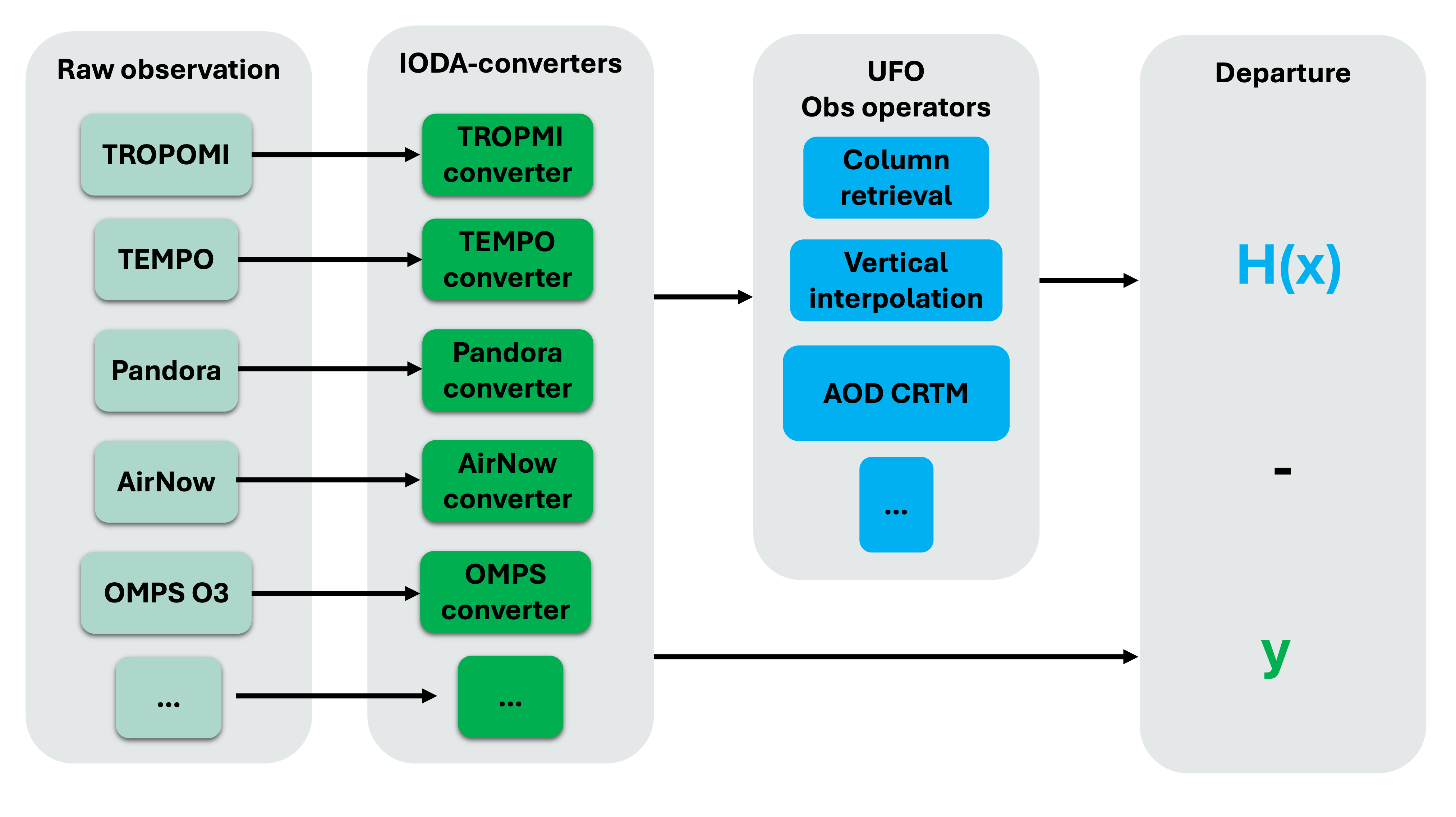
Within JEDI, data in observation space (input observation and output feedback files) are in IODA format.
IODA format is a nested NetCDF with specific Groups that we will explore in this talk.
IODA-converters are written for each observation type to convert raw observation files into the IODA format.

Observation files¶

Let’s take a look at a observation file that is in IODA format:

# Functions used in this lecture:

def print_groups(ioda_filename):
    # Loop through each group in the file
    for group_name in ioda_filename.groups:
        print(f"\n=== Group: {group_name} ===")
    
        group = ioda_filename[group_name]
    
        # List data variables
        if group.data_vars:
            print("  Data variables:")
            for var in group.data_vars:
                print(f"    - {var}")
        else:
            print("  Data variables: None")

import xarray as xr
obs_file = xr.open_datatree('./inputs/tempo_no2_tropo_20230805T150000Z.nc')
print_groups(obs_file)


=== Group: / ===
  Data variables: None

=== Group: /MetaData ===
  Data variables:
    - albedo
    - cloud_fraction
    - dateTime
    - latitude
    - longitude
    - quality_assurance_value
    - solar_zenith_angle
    - viewing_zenith_angle

=== Group: /ObsError ===
  Data variables:
    - nitrogendioxideColumn

=== Group: /ObsValue ===
  Data variables:
    - nitrogendioxideColumn

=== Group: /PreQC ===
  Data variables:
    - nitrogendioxideColumn

=== Group: /RetrievalAncillaryData ===
  Data variables:
    - averagingKernel
    - pressureVertice

Feedback files¶

By running a JEDI H(x) application you can calculate the model equivalent values to your observation using an observation operator. The output of the H(x) run is called a feedback file and is in IODA format. Let’s compare it with the input observation file.

import xarray as xr
live_demo_path = '/discover/nobackup/mabdiosk/JEDI_practicals/live_demo'
fb_file = xr.open_datatree(f'{live_demo_path}/ioda_converters/inputs/fb.hofx3d.tempo_no2_tropo.20230805T150000Z.nc')
print_groups(fb_file)


=== Group: / ===
  Data variables: None

=== Group: /EffectiveError ===
  Data variables:
    - nitrogendioxideColumn

=== Group: /EffectiveQC ===
  Data variables:
    - nitrogendioxideColumn

=== Group: /MetaData ===
  Data variables:
    - cloud_fraction
    - dateTime
    - longitude
    - latitude
    - quality_assurance_value
    - solar_zenith_angle
    - albedo
    - viewing_zenith_angle

=== Group: /ObsBias ===
  Data variables:
    - nitrogendioxideColumn

=== Group: /ObsError ===
  Data variables:
    - nitrogendioxideColumn

=== Group: /ObsValue ===
  Data variables:
    - nitrogendioxideColumn

=== Group: /PreQC ===
  Data variables:
    - nitrogendioxideColumn

=== Group: /RetrievalAncillaryData ===
  Data variables:
    - averagingKernel
    - pressureVertice

=== Group: /hofx ===
  Data variables:
    - nitrogendioxideColumn

The feedback file has additional “Groups” such as EffectiveError, EffectiveQC, and hofx. Similarly, after running a variational application more “Groups” will be added the feedback file such as omb, oma, etc. We will go over these Groups in the future lectures.

IODA converters¶

IODA-converters convert the observation files from their raw format into the IODA format. IODA-converters are written in Python and are typically structured to:

Read raw observation data.
Extract variables and metadata needed by the observation operator or filters.
Apply necessary transformations or unit conversions.
Organize the data into IODA groups.
Write out IODA file using pyioda (Python bindings to the underlying IODA C++ libraries).

You can find many examples of IODA converters in the IODA-converters GitHub repository: https://github.com/jcsda-internal/ioda-converters

More specifically, atmospheric composition converter are in: https://github.com/JCSDA-internal/ioda-converters/tree/develop/src/compo

Let’s take a look at the TROPOMI converter. This converter can handle CO total column, NO2 total column, and NO2 tropospheric column.

It also takes qa_value (optional) as an input to only process pixels with acceptable quality.

Note how the input argument changes between different use cases:

Total CO:

python3 tropomi_no2_co_nc2ioda.py \
  -i inputs/tropomi_co_raw.nc \
  -o outputs/tropomi_co_ioda.nc \
  -v co \
  -q 0.5 \
  -c total

Total NO2:

python3 tropomi_no2_co_nc2ioda.py \
  -i inputs/tropomi_no2_raw.nc \
  -o outputs/tropomi_no2_total_ioda.nc \
  -v no2 \
  -c total

Tropospheric NO2:

python3 tropomi_no2_co_nc2ioda.py \
  -i inputs/tropomi_no2_raw.nc \
  -o outputs/tropomi_no2_trop_ioda.nc \
  -v no2 \
  -c troposphere

For details about setting the environment to run the converter you can review the practical example.

Now let’s compare the IODA files (output of the converter).

import xarray as xr

live_demo_path = '/discover/nobackup/mabdiosk/JEDI_practicals/live_demo'

obs_file = xr.open_datatree(f'{live_demo_path}/ioda_converters/outputs/tropomi_co_ioda.nc')
print('Total CO observation name:')
print(obs_file['ObsValue'].data_vars)
#print_groups(obs_file)

obs_file = xr.open_datatree(f'{live_demo_path}/ioda_converters/outputs/tropomi_no2_total_ioda.nc')
print('Total NO2 observation name:')
print(obs_file['ObsValue'].data_vars)
#print_groups(obs_file)

obs_file = xr.open_datatree(f'{live_demo_path}/ioda_converters/outputs/tropomi_no2_trop_ioda.nc')
print('Tropospheric NO2 observation name:')
print(obs_file['ObsValue'].data_vars)
#print_groups(obs_file)

Total CO observation name:
Data variables:
    carbonmonoxideTotal  (Location) float32 640B ...
Total NO2 observation name:
Data variables:
    nitrogendioxideTotal  (Location) float32 504B ...
Tropospheric NO2 observation name:
Data variables:
    nitrogendioxideColumn  (Location) float32 504B ...

Note how “Groups” and file structure remain the the same but observation variable name is different between these files (carbonmonoxideTotal, nitrogendioxideTotal, nitrogendioxideColumn).

IODA format follows the JEDI naming conventions for naming the variables. You can see the full list here.

Ctest in IODA-converters¶

Each converter in the IODA-converters repository has a dedicated unit test that is there to ensure the converter is working properly. The ctests can also be used as references to learn how the converters run, what are the required inputs, and what the outputs look like. Let’s take a look at the TROPOMI CO ioda converter.

In ioda-converters/test/CMakeLists.txt find where TROPOMI CO test is added:

ecbuild_add_test( TARGET  test_${PROJECT_NAME}_tropomi_co_total
                  TYPE    SCRIPT
                  ENVIRONMENT "PYTHONPATH=${IODACONV_PYTHONPATH}"
                  COMMAND bash
                  ARGS    ${CMAKE_BINARY_DIR}/bin/iodaconv_comp.sh
                          netcdf
                          "${Python3_EXECUTABLE} ${CMAKE_BINARY_DIR}/bin/tropomi_no2_co_nc2ioda.py
                          -i testinput/tropomi_co.nc
                          -o testrun/tropomi_co_total.nc
                          -v co
                          -q 0.5
                          -c total"
                          tropomi_co_total.nc ${IODA_CONV_COMP_TOL})

In the next lecture we go over different observation operators and running a simple H(x) application.